Exploring NLP with Coursera - Part 4
During Week 1, I realised that taking notes that mimic the content doesn’t make sense as much, thus for Week 2, the notes cover only highlights and important outcomes.
Basics of Language Modeling
Let’s say we have the text “This is the…” and 4 possible choices
- house
- rat
- did
- malt
For humans, this might not be a trivial question and we could say that for example did doesn’t really fit here in any context. For machines, its a bit more challenging.
We can help machines to “understand” better using probability theory. For example, what is the probability of seeing the word ‘house’ given ‘this is the’ or
\[p(house|this\ is\ the)\]In terms of language modeling we can also ask the probability of the whole sequence. Given our training data how likely are we to see a specific sequence. For example
\[p(this\ is\ the\ house)\]Mathematically, we want to predict the probability of a sequence of words This is the house, which we can annotate as
\[w=(w_1w_2w_3...w_k)\]Thus the probability of it would be
\[p(w)=p(w_1w_2w_3...w_k)\]Using the Chain Rule we can rewrite the equation as such
\[p(w)\ =\ p(w_1)p(w_2|w_1)...p(w_k|w_1...w_{k-1})\]Now the challenge here is that the list of probabilities will explode exponentially making it almost impossible to estimate probabilities. Nevertheless, we can use the Markov Assumption to only take the last n-1 terms. So if we want to look at trigrams then we would condition our probabities on last 2 items in the sequence.
Using Markov Assumption we get
\[p(w_i|w_1...w_{i-1})=p(w_i|w_{i-n+1}...w_{i-1})\]Now, if we use the following probability calculation to our individual probabilities won’t add to one and for that we need to add additional start and end tokens to answer the question what is the probability of seeing specific word given its the start and end of the sequence.
\[p(w_1|start)\]This helps us normalize the probabilities for each sequence.
Thus at the for a n-gram Language Model we have the following representation
\[p(w)=\prod_{i=1}^{k+1}p(w_i|w_{i-n+1}^{i-1})\]
and the model estimate is simply the countings for those word representations

To train the N-gram Language Model, we simply maximize the log likelihood

The large N represents the length of the train corpus (all words concatenated)
Smoothing: Dealing with un-seen n-grams
Now there will be situations where in the test data we observe text (n-grams) that is not present in the training data, essentially leading to zero probabilities. To deal with these situations, various smoothing techniques could be used.
Essentially smoothing tries to pull some probability from frequent n-grams to infrequent ones.
Let’s review various smoothing techniques. This section is pretty straight forward since it simply summarizes various approaches.
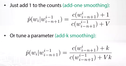
Laplacian Smoothing
Katz Backoff
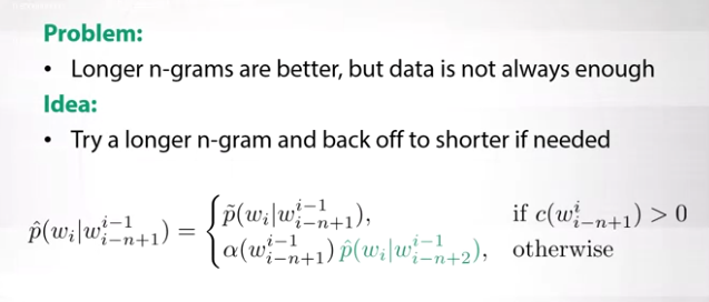
Here and p and alpha are chosen to ensure normalization.
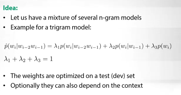
Interpolation Smoothing
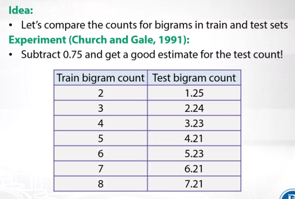
Absolute Discounting
The approach was developed as a result of the experiment made by Church & Gale in 1991. Experiment available here.

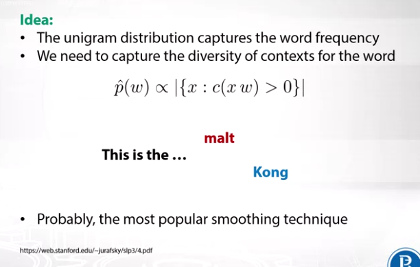
Kneser-Ney Smoothing
This smoothing technique is the most popular smoothing technique mostly because it captures the diversity of contexts for the word. Example here is that the word Kong is less likely to occur with This is the… because it only goes with Hong Kong but the word malt can be seen in various context, thus more likely to be preceded by This is the.

Perplexity Computation
Perplexity is a popular quality measure of language models. We can calculate it using the formula:
There is a nice short article on what Perplexity here.